We developed TIPS (Transcriptional Instability Prediction of Subnetworks) to better
understand birth defects by (i) testing the “controlled chaoticity” hypothesis at the
transition (ordered connectivity + targeted fragility), and (ii) prioritizing mechanistic
bridge/hub genes and downstream “dual‑pull” architecture underlying the developmental
bifurcation.
test the “controlled chaoticity” hypothesis at the transition
(ordered connectivity + targeted fragility), and
prioritize mechanistic bridge/hub genes and downstream “dual-pull”
structure for the CP → (CM vs CF-like) bifurcation.
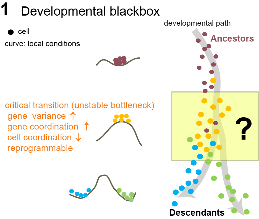
Figure 1: A cell begins in a single stable state. As new fate programs emerge,
their competing influences pull the system into a highly dynamic transition region where multiple states are explored.
The balls and hills represent changes in the underlying potential landscape that shape how easily the cell can move between states.
The cell then settles into one of several stable phenotypic outcomes.
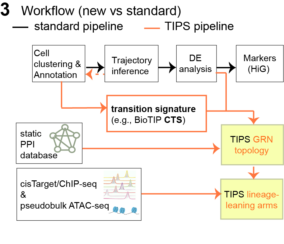
2. TIPS workflow: continuing from BioTIP (Fig 2)
BioTIP answers “where is the tipping point and what genes
define it?” → by identifying critical transition clusters and their CTS
modules (instability peak).
TIPS answers “how is that CTS organized mechanistically
and how vulnerable is it?” → by mapping dynamic CTS (and CTS&HiG) onto a
static protein–protein interaction (PPI) scaffold, then weighting edges
using cluster-specific coexpression.
TIPS integrates two inputs: 1) BioTIP critical-transition outputs (CTS), historical
markers (highly expressed genes, HiG), and their overlap (CTS&HiG); 2) a static
PPI with knowledge-based edge weights.
TIPS outputs three categories of cluster-specific, edge‑weighted protein–protein
interaction networks (PPINs) (i.e., static knowledge-based PPI backbone × data-
driven cluster‑specific coexpression specificity).
Figure 2: How BioTIP and TIPS analysis fit into overall cell-state discovery and differentiation trajectory pipeline.
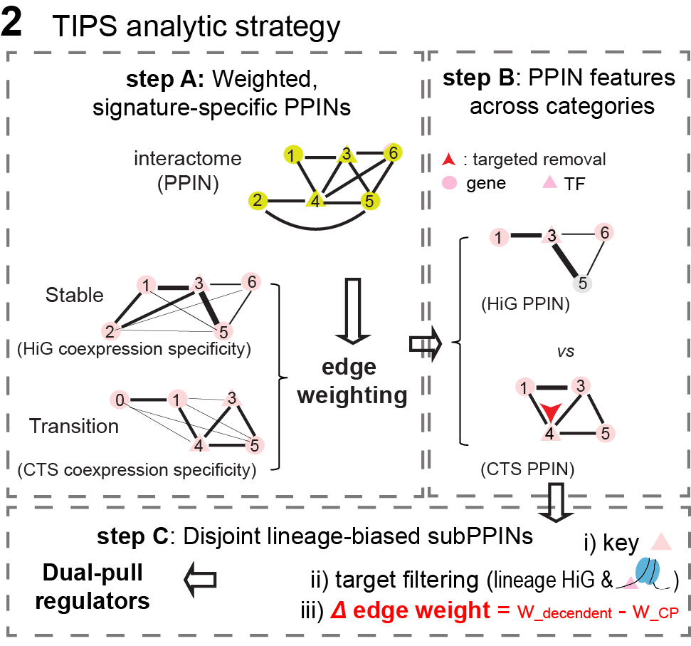
3. TIPS two-step analytic strategy and key concepts (Fig 3)
There are two steps:
In Step A, curated, knowledge based interactome is restricted to genes in a cluster
specific signature to form a signature derived subnetwork. STRING interaction
support is then combined with cluster specific coexpression information to assign
state specific edge weights, yielding a weighted protein–protein interaction network
(PPIN) for each cell state, where genes are nodes and weighted interactions represent
a combination of protein–protein associations and coexpression specificity.
In Step B, the weighted PPINs are analyzed for topological properties and
robustness via strategic node removal (red arrows). Robustness is quantified and
compared among three categories of PPINs: stable (HiG), transitional (CTS), and
their overlap (CTS&HiG) networks.
Like BioTIP, TIPS can use shrinkage correlation
(stabilizes correlation estimates and reduces spurious correlations in
smaller/noisier clusters).
TIPS then adds an explicit specificity penalty
|rtarget| × (1 − mean(|rother|))
so ubiquitous coexpression (often driven by broadly expressed or highly
expressed programs) is downweighted, while cluster-selective coupling
is emphasized.
Coexpression magnitude uses the absolute value (direction-agnostic
strength), while the sign is stored separately for visualization (positive vs
negative edges).
Figure 3: Overview of TIPS analysis including how PPINS are constructed,
how edges are updated, and how robustness is tested through targeted node attacks.
We reanalyzed and applied BioTIP to the E8.25 subsets and demonstrated the
robustness of BioTIP identification across multiple datasets, including
this subset (Figure S1 in Yang et al., 2022).
We previously built a BioTIP tutorial using this dataset
[URL].
Specifically, raw counts and metadata were obtained from the
MouseGastrulationData R package. We extracted E8.25 cells and
removed cells annotated as putative doublets or stripped nuclei as
described in our prior reanalysis (Yang et al., 2022), yielding 7,240
E8.25 mesoderm cells.
Counts were normalized with scran::logNormCounts using
sample-specific size factors. Gene selection and clustering followed
Yang et al. (2022): PCA was performed on the selected expressed-gene set,
and clusters were identified using an SNN graph (k = 10)
and graph-based clustering, resulting in 19 subpopulations.
Cluster markers were identified using
SingleCellExperiment::findMarkers
(t-test; logFC > 0.6; min.prop = 0.25; FDR < 0.01).
Following, we detail the main delivery of TIPS analysis presented in the following
Figure by walking through the R set up, and each panel – the purpose, R code,
interpretation, inputs and outputs.
TIPS Walkthrough
Main Figure: Polished figure generated by TIPS workflow.
Setup
Load libraries & initialize global variables
library(gplots)
require(dplyr)
library(data.table)
library(ggplot2)
library(ggpubr)
library(ggrepel)
library(igraph)
library(rstatix)
library(scales)
library(pracma)
library(MLmetrics)
library(sm)

########## BEGINNING OF USER INPUT ##########

wd = "/Users/felixyu/Documents/GSE87038_weighted/" # working directory
celltype_specific_weight_version <- '10'
source(paste0('https://raw.githubusercontent.com/xyang2uchicago/TIPS/refs/heads/main/R/celltype_specific_weight_v', celltype_specific_weight_version, '.R')) # source from GitHub or use local file

db <- "GSE87038" # dataset name for file naming

PPI_color_palette = c("CTS" = "#7570B3", "HiGCTS" = "#E7298A", "HiG" = "#E6AB02") # Coloring for HiG, HiGCTS, and HiG clusters
PPI_size_palette = c("CTS" = 1, "HiGCTS" = 0.75, "HiG" = 0.25) # Line width for HiG, HiGCTS, and HiG clusters

CT_id = c("7", "8", "11", "13", "15", "16", "16.1") # critical transition cluster ids
CT_id_formatted <- paste0("_(", paste(CT_id, collapse = "|"), ")")


setwd(paste0(wd, 'results/PPI_weight/'))
inputdir = "../../data/" # directory for input data files (e.g. CHD_Cilia_Genelist.rds)

# For Figure E
# Choose what to plot: "vertex", "edge", or "both"
plot_mode <- "vertex"  # change this to "edge" or "both" as needed

# For Figure K
CP_CTS <- "HiGCTS_8" # cardiac progenitor critical transition cluster

s = "combined" # specificity method

########## END OF USER INPUT ##########

file = paste0(db, '_STRING_graph_perState_simplified_',s,'weighted.rds')
graph_list <- readRDS(file)

(names(graph_list))
#  [1] "HiG_1"       "HiG_2"       "HiG_3"       "HiG_4"       "HiG_5"       "HiG_6"       "HiG_9"       "HiG_10"      "HiG_12"      "HiG_14"      "HiG_17"      "HiG_18"      "HiG_19"      "HiG_7"
# [15] "HiG_11"      "HiG_15"      "HiG_16"      "HiG_13"      "HiG_8"       "HiGCTS_7"    "HiGCTS_11"   "HiGCTS_15"   "HiGCTS_16"   "HiGCTS_16.1" "HiGCTS_8"    "CTS_7"       "CTS_11"      "CTS_15"
# [29] "CTS_16"      "CTS_16.1"    "CTS_13"      "CTS_8"       "HiGCTS_13"

signature_levels = c(names(graph_list))
Panel A & Panel B — Strength Architecture and Distribution
Purpose
To evaluate the weighted connectivity structure of each PPIN derived from GSE87038 signatures.
Normalized node strength reflects the sum of all weighted interactions per gene,
adjusted for network size. These panels describe both the typical strength
(medians) and the full distribution across categories
(CTS, CTS&HiG, HiG).
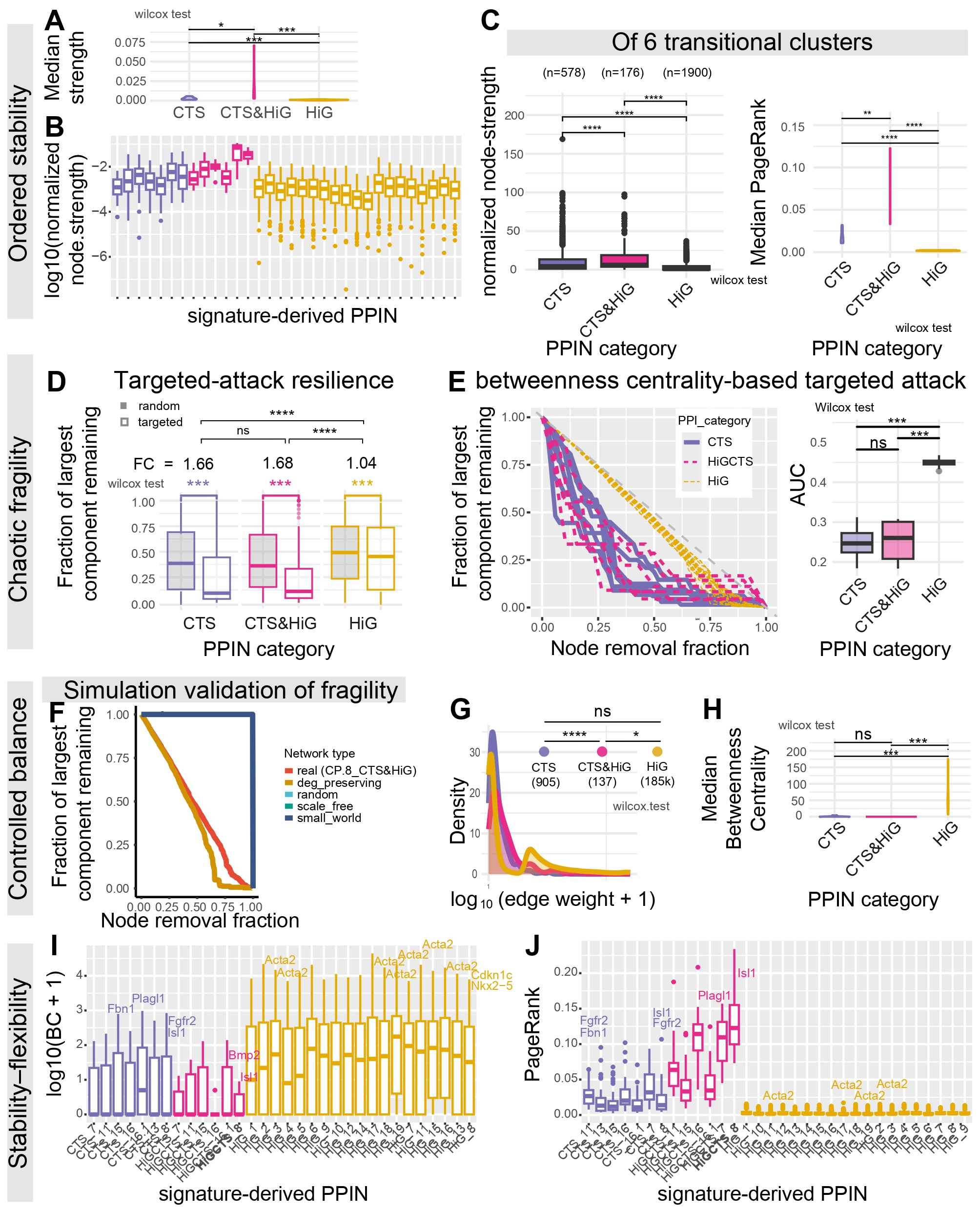
What this Panel Shows
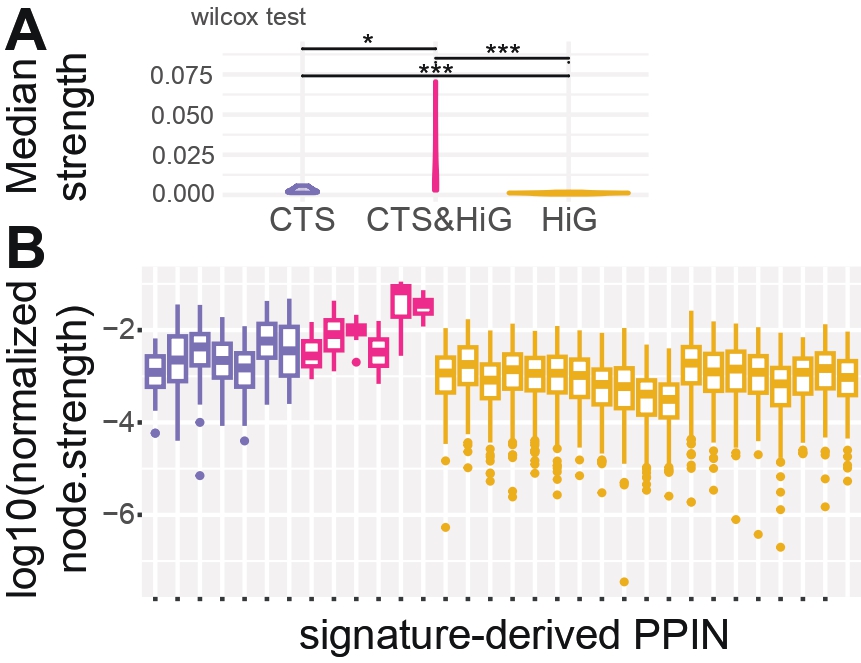
A: Summarized on PPIN category level, median normalized node strength (violin plot). Each point is a PPIN’s median.
Violin shapes show the distribution of medians within each category.
Wilcoxon tests compare CTS vs CTS&HiG, CTS&HiG vs HiG, CTS vs HiG.
B: Detailed on cluster level, boxplot of normalized node strength for all genes (log₁₀ scale).
CHD-risk genes labeled if top 5 strongest.
Interpretation
Despite being a much smaller overlap set, CTS&HiG PPINS contain higher normalized connection strength between nodes.
Inputs
df_PAGERANK_strength_ANND.rewring.P.rds
CHD_Cilia_Genelist.rds
graph_list from GSE87038_STRING_graph_perState_simplified_combinedweighted.rds
Outputs
Note: figures shown are polished versions of the raw outputs
Code
Top
###################################################
# Fig A ) normalized node strength analysis
# original code: 11.3_CTS_cardiac_network_ANND_pagerank.R
# original pdf: normalized.node.strength_GSE87038_v2.pdf
################################################################
{
df = readRDS(file='df_PAGERANK_strength_ANND.rewring.P.rds')  #!!!!!!!!!!!!!!!!!!!!!!!
df = rbind(subset(df, PPI_cat=='CTS'),
                    subset(df, PPI_cat=='HiGCTS'),
                    subset(df, PPI_cat=='HiG')
                    )
df$label=df$gene

CHD = readRDS( file=paste0(inputdir, 'CHD_Cilia_Genelist.rds'))

df_median = df %>% group_by(signature) %>%
                    summarise(median_normalized_strength = median(normalized.strength, na.rm = TRUE))
df_median$PPI_cat = lapply(df_median$signature, function(x) unlist(strsplit(x, split='_'))[1]) %>% unlist
df_median$PPI_cat = factor(df_median$PPI_cat,levels=c('CTS', 'HiGCTS', 'HiG'))

violin_median_normalized.strength_wilcox = ggplot(df_median, aes(x = PPI_cat, y = median_normalized_strength, color = PPI_cat, fill = PPI_cat)) +
        geom_violin(alpha = 0.3) +  # Violin plot with transparency
        scale_color_manual(values = PPI_color_palette) +
        scale_fill_manual(values = PPI_color_palette) +
        theme_minimal() +
        theme(legend.position = "none") + #, axis.text.y = element_blank(), axis.title.y = element_blank()) +
        labs(x = "PPI category", y = "median of normalized node strength per PPI") +  # Label the axes
        # Add statistical comparisons using stat_compare_means
        stat_compare_means(
        aes(group = PPI_cat),  # Grouping by the 'PPI_cat' column
        comparisons = list(c("HiG", "CTS"), c("HiG", "HiGCTS"), c("HiGCTS", "CTS")),  # Specify comparisons
        method = "wilcox.test",  # Non-parametric test (Wilcoxon)
        label = "p.signif",  # Show significance labels (e.g., **, *, ns)
        label.x = 1.5,  # Adjust x-position of the p-value text
        size = 4  # Adjust size of the p-value text
        ,tip.length =0
        ) +
ggtitle('wilcox, median nor_strength')
vertex(violin_median_normalized.strength_wilcox)
}
Bottom
###################################################
# Fig B) boxplot of normalized strength for all clusters per category
# original code: 11.3_CTS_cardiac_network_ANND_pagerank.R
# original pdf: normalized.node.strength_GSE87038_v2.pdf
################################################################
{
CHD = readRDS(file = paste0(inputdir, "CHD_Cilia_Genelist.rds"))

df = readRDS(file = "df_PAGERANK_strength_ANND.rewring.P.rds")

# Keep only desired PPI categories in the correct order
df = rbind(
    subset(df, PPI_cat == "CTS"),
    subset(df, PPI_cat == "HiGCTS"),
    subset(df, PPI_cat == "HiG")
)

# Enforce the factor order
df$PPI_cat = factor(df$PPI_cat, levels = c("CTS", "HiGCTS", "HiG"))
df$signature = factor(df$signature, levels = unique(df$signature))

# Add CHD gene annotations
df$PCGC_AllCurated = toupper(df$gene) %in% toupper(unlist(CHD["Griffin2023_PCGC_AllCurated"]))

# Identify top 5 genes per signature by normalized strength
top_genes = df %>%
    group_by(signature) %>%
    arrange(desc(normalized.strength)) %>%
    slice_head(n = 5) %>%
    ungroup()

# Subset top CHD genes
top_genes_CHD = subset(top_genes, PCGC_AllCurated == TRUE)
(dim(top_genes_CHD))  # Optional: check how many CHD genes were top 5

# Optional: write out table of top 5 genes
tb = top_genes[, c("signature", "gene", "PPI_cat", "normalized.strength", "PCGC_AllCurated")]
write.table(tb, file = "table_top5_strength_perPPI.tsv", sep = "\t", row.names = FALSE)

# Plot
boxplot_strength = ggplot(df, aes(x = signature, y = log10(normalized.strength), colour = PPI_cat)) +
    geom_boxplot(show.legend = TRUE, position = position_dodge2(preserve = "single")) +
    scale_color_manual(values = PPI_color_palette) +
    geom_text_repel(
        data = top_genes_CHD,
        aes(label = gene),
        size = 2,
        box.padding = 0.5,
        point.padding = 0.5,
        segment.color = "grey50",
        max.overlaps = 20,
        show.legend = FALSE
    ) +
    theme(
        legend.position = "none",
        legend.justification = c(1, 1),
        axis.text.x = element_text(angle = 45, vjust = 1, hjust = 1)
    ) +
    scale_x_discrete(limits = unique(df$signature)) +
    labs(color = "PPI cat")

vertex(boxplot_strength)
}
Panel C — Connectivity and PageRank Influence of Transition-Cluster PPINs
Purpose
Node-strength: To determine whether PPINs derived from transcriptionally unstable
critical transition signatures (CTSs) (clusters 7, 8, 11, 13, 15, 16, 16.1)
show systematically altered connectivity.
PageRank:
To quantify how global influence is distributed within each CTS PPIN. PageRank identifies genes
positioned on influential, central information routes through the network.
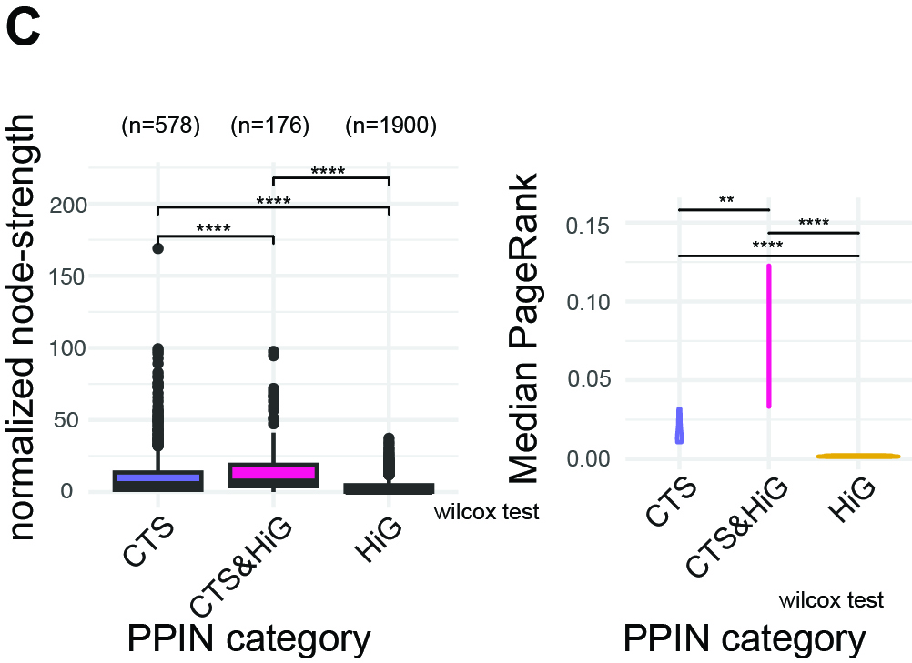
What this Panel Shows
Node-strength: A boxplot of normalized node strength for PPINs from transition clusters,
grouped into CTS, CTS&HiG, and HiG categories.
PageRank: A violin plot of the median PageRank per PPIN across CTS, CTS&HiG, and HiG.
Wilcoxon tests quantify pairwise differences.
Interpretation
CTS&HiG networks exhibit higher normalized node strength and higher median PageRank than HiG,
particularly when limited to just the six transition clusters.
Because strength is normalized for network size and PageRank reflects relative centrality,
these results indicate that CTS&HiG nodes remain densely connected and centrally positioned.
Inputs
graph_list from GSE87038_STRING_graph_perState_simplified_combinedweighted.rds
df_PAGERANK_strength_ANND.rewring.P.rds
Outputs
Note: figures shown are polished versions of the raw outputs
###################################################
# Fig D) violin plot of median PageRank per category
# original code: 11.3_CTS_cardiac_network_ANND_pagerank.R
# original pdf: PageRank_IbarraSoria20183_v2.pdf
################################################################
{
df = readRDS(file='df_PAGERANK_strength_ANND.rewring.P.rds')  #!!!!!!!!!!!!!!!!!!!!!!!
df = rbind(subset(df, PPI_cat=='CTS'),
                    subset(df, PPI_cat=='HiGCTS'),
                    subset(df, PPI_cat=='HiG')
                    )
df$label=df$gene

df_median = df %>% group_by(signature) %>%
                    summarise(pg.median = median(PageRank, na.rm = TRUE))
df_median$PPI_cat = lapply(df_median$signature, function(x) unlist(strsplit(x, split='_'))[1]) %>% unlist
df_median$PPI_cat = factor(df_median$PPI_cat,levels=c('CTS', 'HiGCTS', 'HiG'))

violin_median_pagerank = ggplot(df_median, aes(x = PPI_cat, y = pg.median, color = PPI_cat, fill = PPI_cat)) +
        geom_violin(alpha = 0.3) +  # Violin plot with transparency
        scale_color_manual(values = PPI_color_palette) +
        scale_fill_manual(values = PPI_color_palette) +
        theme_minimal() +
        theme(legend.position = "none") + #, axis.text.y = element_blank(), axis.title.y = element_blank()) +
        labs(x = "PPI category", y = "median of PageRanks per PPI") +  # Label the axes
        # Add statistical comparisons using stat_compare_means
        stat_compare_means(
        aes(group = PPI_cat),  # Grouping by the 'PPI_cat' column
        comparisons = list(c("HiG", "CTS"), c("HiG", "HiGCTS"), c("HiGCTS", "CTS")),  # Specify comparisons
        method = "wilcox.test",  # Non-parametric test (Wilcoxon)
        label = "p.signif",  # Show significance labels (e.g., **, *, ns)
        label.x = 1.5,  # Adjust x-position of the p-value text
        size = 4  # Adjust size of the p-value text
        ,tip.length =0
        ) +
        ggtitle('wilcox test, median PA')

vertex(violin_median_pagerank)
}
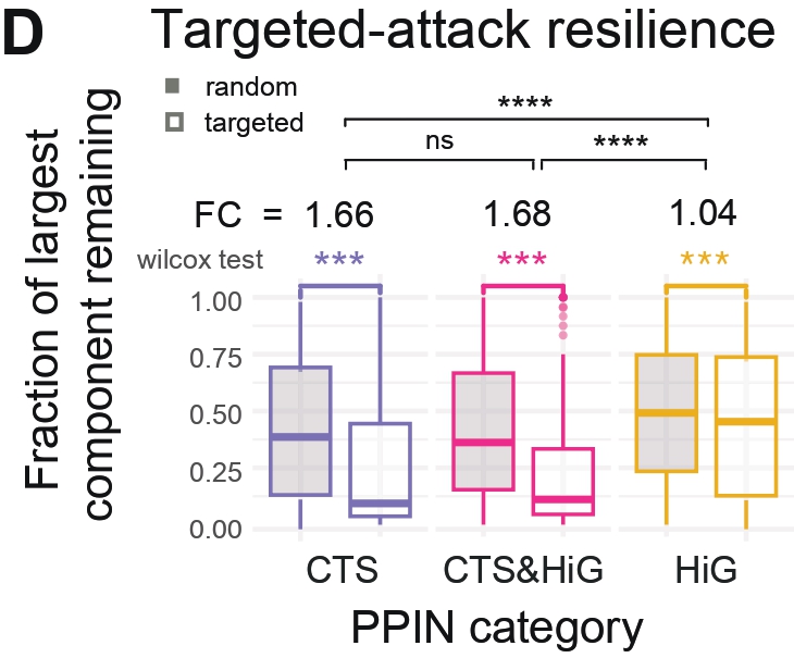
Panel D — Resistance to Targeted and Random Attacks
Purpose
To test PPIN robustness under random failure vs targeted removal of high-betweenness nodes.
What this Panel Shows
Boxplots of the remaining fraction of the largest connected component
under random vs targeted removal.
Faceted by CTS / CTS&HiG / HiG.
Wilcoxon tests compare severity of collapse.
Interpretation
When nodes were removed by descending betweenness centrality, CTS and CTS&HiG
PPINs fragmented faster than HiG PPINs, whereas random removal had a much weaker
effect in the transition PPINS.
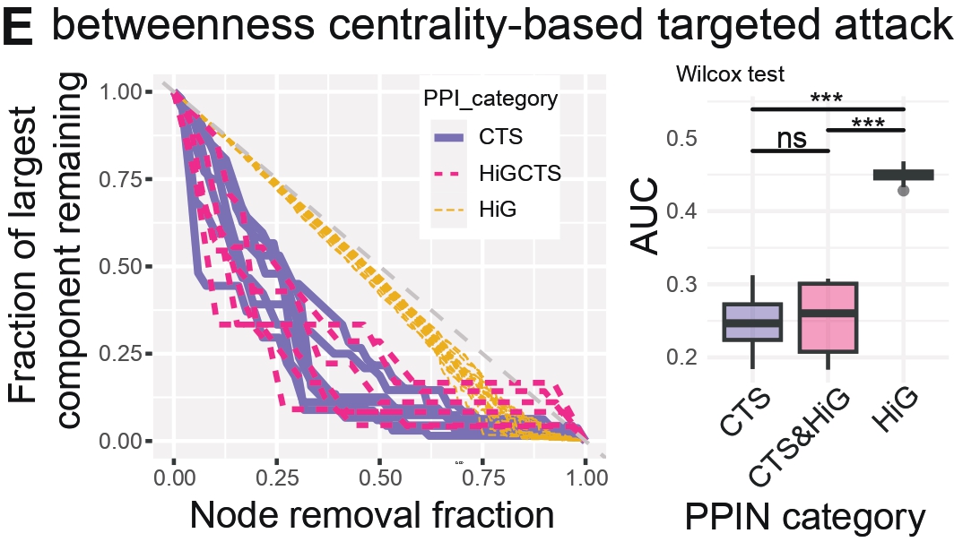
Panel E — Fragmentation Trajectories and Robustness AUC
Purpose
To quantify PPIN robustness under targeted vertex removal by observing how networks fragment as key nodes are deleted.
Robustness is quantified by tracking network fragmentation (e.g., loss of the largest connected component) under strategic
versus random removal, enabling comparison of PPIN vulnerability across categories.
What this Panel Shows
Left: Fragmentation curves — Tracks the collapse of each PPIN under targeted node removal.
Plots the percentage of nodes removed vs. the remaining size of the largest connected component.
Curves colored by PPI category reveal whether PPINs fragment early (steep curves) or remain intact longer (flatter curves).
Right: AUC boxplots — The Area Under the Curve summarizes PPIN robustness.
Higher AUC indicates greater robustness (i.e., resilience to targeted node removal).
Interpretation
Low AUC → fragile networks that collapse early under targeted attacks. High AUC → robust networks that maintain connectivity longer.
Transition PPINs show significantly lower AUC, indicating heightened vulnerability to the removal
of influential nodes and fewer redundant paths relative to HiG networks.
###################################################
# Fig H) boxplot of AUC for vertex attack
# original code: 11.2_CTS_cardiac_network_robustness.R
# original pdf: box_wilcox-test_attack_AUC_GSE87038.pdf
################################################################
{
failure.dt = readRDS(file=paste0('failure.vertex_100_simplified_', s, 'weighted.rds'))
colnames(failure.dt)[1] = 'signature'

attack.vertex.btwn = readRDS('attack.vertex.btwn.rds')
colnames(attack.vertex.btwn)[1] = 'signature'

robustness.dt <- rbind(failure.dt, attack.vertex.btwn[,1:6])
robustness.dt$PPI_cat = lapply(robustness.dt$signature, function(x) unlist(strsplit(x , '_'))[1]) %>% unlist %>%
    factor(.,levels=c('CTS', 'HiGCTS', 'HiG'))

robustness.dt = subset(robustness.dt ,measure != 'degree')
robustness.dt$type = factor(robustness.dt$type,
    levels = c("Random edge removal","Targeted edge attack","Random vertex removal","Targeted vertex attack"))

observed_auc_list = list()
for(j in names(graph_list)){
	observed_auc_list[[j]] = Area_Under_Curve(subset(robustness.dt, signature==j & type=='Targeted vertex attack')$removed.pct,
				 subset(robustness.dt, signature==j & type=='Targeted vertex attack')$comp.pct )
}
df_AUC = data.frame(auc=observed_auc_list %>% unlist,
			signature = names(observed_auc_list),
			PPI_cat = lapply(names(observed_auc_list), function(x) unlist(strsplit(x, split='_'))[1]) %>% unlist)
df_AUC$PPI_cat  = factor(df_AUC$PPI_cat , levels = c('CTS',"HiGCTS" ,"HiG"))

boxplot_AUC_vertex_attack = ggplot(df_AUC, aes(x = PPI_cat, y = auc, fill = PPI_cat)) +
  geom_boxplot(alpha = 0.5, position = position_dodge(width = 0.75)) +  # Dodge the boxes for each type per PPI_cat
  #facet_wrap(experiment ~ PPI_cat, ncol = 3) +  # Facet by PPI_cat, each PPI_cat gets a row
  scale_fill_manual(values = PPI_color_palette) +
  #scale_fill_manual(values = c("random" = "grey", "btwn.cent" = "orange")) +
  geom_signif(
    comparisons = list(
      c("CTS", "HiGCTS"), c("HiGCTS", "HiG"),c("CTS", "HiG")
    ),
    map_signif_level = TRUE,
    step_increase = 0.1,  # Adjusts spacing between the lines
    #aes(group = type),
    test = "wilcox.test"  # Perform a t-test to calculate significance
	#, p.adjust.method = "holm"   # default is
  ) +
  theme_minimal() +
  labs(
    title = "Comparison of Robustness Measures by cent.btw",
    x = "PPI Category",
    y = "AUC of targeted vertex attack"
  ) +
  theme(legend.position = "top")
vertex(boxplot_AUC_vertex_attack)
}
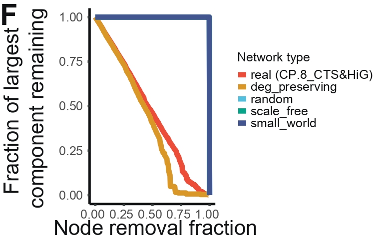
Panel F — Simulation Network Fragility
Purpose
To compare empirical PPIN fragility against synthetic network models generated from standard
topological frameworks. Monte-Carlo simulations test whether the vulnerability of real CTS/HiG networks
arises from their degree structure or reflects deeper organizational constraints.
What this Panel Shows
Left: Simulation-based fragmentation curves — Plots the remaining size of the largest
connected component as nodes are progressively removed, across multiple network types:
Real PPINs (CTS + HiG)
Degree-preserving randomized networks
Fully random networks
Scale-free networks
Small-world networks
Right: Bar plot of AUC values — Summarizes robustness for each network class.
Higher AUC corresponds to greater resilience against node removal.
Together, the simulations determine whether empirical PPIN fragility can be explained by simple degree structure or requires more complex biological organization.
Interpretation
The simulation graph shows that degree-preserving rewired CTS&HiG networks lose global connectivity
earlier than the real PPIN, indicating that resilience is not explained by the degree sequence alone
but depends on biologically structured edge placement. At the same time, the real network fragments
earlier than toy generative graphs, placing CTS&HiG PPINs in an intermediate regime that balances robustness
to random disruption with selective vulnerability to targeted bridge removal.
Inputs
graph_list from GSE87038_STRING_graph_perState_simplified_combinedweighted.rds
Outputs
Note: figures shown are polished versions of the raw outputs
###################################################
# Fig K) Monte-Carlo robustness simulation for CP_CTS
# original code: 11.7_synthetic_simulation.R
# original pdf: simulation.pdf
###################################################
{
# Select real network
g_real <- graph_list[[CP_CTS]]

# Run simulation
res <- synthetic_simulation(g_real, main = CP_CTS)

# Combine into a single plot object
plot_simulation <- grid.arrange(
    res$p_weights,
    res$p_line,
    res$p_AUC,
    ncol = 3
)

print(plot_simulation)
}
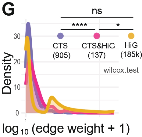
Panel G — Distribution of PPI Edge Weights
Purpose
To compare how strongly connected the protein–protein interactions (PPINs) are
within each PPIN category (CTS, CTS&HiG, HiG). Edge weight is a combination of
string PPI confidence and coexpression in that cluster.
What this Panel Shows
Kernel density curves of log10(edge weight + 1) for each PPI category.
Pairwise Wilcoxon tests (CTS vs CTS&HiG, CTS vs HiG, CTS&HiG vs HiG) with significance annotations.
The number of edges used for each category is shown under each label.
Interpretation
Modules are tightly connected groups of nodes; since all network categories have similar numbers of modules,
their different fragilities must arise from how modules are wired together, not from how many modules exist.
Inputs
GSE87038_STRING_graph_perState_notsimplified.rds
correct_n_edges_HiG_STRING2.14.0.rds
Edge weights extracted with extract_edge_weights_by_category()
Plotted with plot_edge_weight_distributions()
Outputs
Note: figures shown are polished versions of the raw outputs
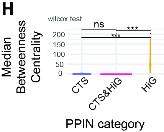
To evaluate whether PPIN categories differ in bottleneck load, using betweenness
centrality to identify nodes that lie on many shortest paths.
What this Panel Shows
Violin plots of the median betweenness per PPIN across categories.
Interpretation
At the category level, median betweenness centrality is significantly lower in CTS and CTS&HiG PPINs
compared with HiG PPINs. This indicates that HiG networks are more dominated by a small number of
high-betweenness hub nodes, whereas transition PPINs (CTS and CTS&HiG) exhibit a more distributed
topology with fewer globally dominant bottlenecks. In other words, information flow in HiG PPINs is
concentrated through central hubs, while transition PPINs spread connectivity more evenly across nodes.
Inputs
df_betweeness.tsv
Outputs
Note: figures shown are polished versions of the raw outputs
###################################################
# Fig G) violin plot of median betweenness per category
# original code: Code: 11.3_CTS_cardiac_network_ANND_pagerank.R
# original pdf: BetweennessCentrality_GSE870383_v2.pdf
################################################################
{
df_BC = read.table(file='df_betweeness.tsv',sep='\t', header=T)
df_BC$PPI_cat = factor(df_BC$PPI_cat,levels=c('CTS', 'HiGCTS', 'HiG'))
df5 <- df_BC %>%
        filter(rank_by_BC <= 5 & BetweennessCentrality>0) %>%
        ungroup()

df_median = df_BC %>% group_by(signature) %>%
                    summarise(bc.median = median(BetweennessCentrality, na.rm = TRUE)) %>%
                    as.data.frame()
df_median$PPI_cat = lapply(df_median$signature %>% as.vector, function(x) unlist(strsplit(x, split='_'))[1]) %>% unlist
df_median$PPI_cat = factor(df_median$PPI_cat,levels=c('CTS', 'HiGCTS', 'HiG'))

violin_median_bc_wilcox = ggplot(df_median, aes(x = PPI_cat, y = bc.median , color = PPI_cat, fill = PPI_cat)) +
        geom_violin(alpha = 0.3, drop = FALSE) +  # Violin plot with transparency
        scale_color_manual(values = PPI_color_palette) +
        scale_fill_manual(values = PPI_color_palette) +
        theme_minimal() +
        theme(legend.position = "none") + #, axis.text.y = element_blank(), axis.title.y = element_blank()) +
        labs(x = "PPI category", y = "median of BC per PPI") +  # Label the axes
        # Add statistical comparisons using stat_compare_means
        stat_compare_means(
        aes(group = PPI_cat),  # Grouping by the 'PPI_cat' column
        comparisons = list(c("HiG", "CTS"), c("HiG", "HiGCTS"), c("HiGCTS", "CTS")),  # Specify comparisons
        method = "wilcox.test",  # Non-parametric test (Wilcoxon)
        label = "p.signif",  # Show significance labels (e.g., **, *, ns)
        label.x = 1.5,  # Adjust x-position of the p-value text
        size = 4  # Adjust size of the p-value text
        ,tip.length =0
        ) +
        ylim(0, NA)  +  # Start from 0, let ggplot choose upper limit
        ggtitle('wilcox-test, median BC')

plot(violin_median_bc_wilcox)
}
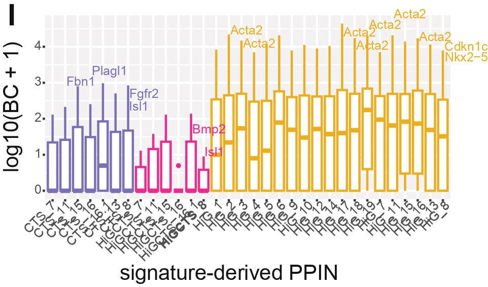
Panel I — Boxplot of Betweenness per PPIN
Purpose
To visualize the full distribution of betweenness centrality across all genes in each PPIN,
complementing Panel H.
What this Panel Shows
Boxplot of log₁₀(betweenness + 1) per PPIN, colored by category.
CHD-risk genes labeled when they appear in the top 5 betweenness-ranked nodes.
Interpretation
Although transition PPIN categories have lower median betweenness overall (as seen in H),
individual CTS and CTS&HiG PPINs display a pronounced upper tail of nodes with high betweenness centrality.
These nodes act as structural bridges linking otherwise weakly connected modules within the network.
The presence of such high-BC outliers indicates “few-node sensitivity”: while the network is broadly distributed,
it remains vulnerable to perturbation of a small set of key bridge nodes. This motivates gene-level prioritization
within transition PPINs, as these nodes disproportionately maintain inter-module communication.
Inputs
df_betweeness.tsv
CHD_Cilia_Genelist.rds
Outputs
Note: figures shown are polished versions of the raw outputs
###################################################
# Fig I) boxplot of betweenness per PPIN
# original code: Code: 11.3_CTS_cardiac_network_ANND_pagerank.R
# original pdf: BetweennessCentrality_IbarraSoria2018_v2.pdf
################################################################
{
df_BC <- read.table(file = "df_betweeness.tsv", sep = "\t", header = T)
df_BC$PPI_cat <- factor(df_BC$PPI_cat, levels = c("CTS", "HiGCTS", "HiG"))

CHD <- readRDS(file = paste0(inputdir, "CHD_Cilia_Genelist.rds"))
df_BC$PCGC_AllCurated <- toupper(df_BC$gene) %in% toupper(unlist(CHD["Griffin2023_PCGC_AllCurated"]))

# Calculate top 5 significant genes within each box
df5 <- df_BC %>%
    filter(rank_by_BC <= 5 & BetweennessCentrality > 0) %>%
    ungroup()

df5_CHD <- subset(df5, PCGC_AllCurated == TRUE)

df_BC <- rbind(
    subset(df_BC, PPI_cat == "CTS"),
    subset(df_BC, PPI_cat == "HiGCTS"),
    subset(df_BC, PPI_cat == "HiG")
)
df_BC$signature <- factor(df_BC$signature, levels = unique(df_BC$signature))

boxplot_bc_log10 <- ggplot(df_BC, aes(x = signature, y = log10(BetweennessCentrality + 1), colour = PPI_cat)) +
    geom_boxplot(position = "dodge2") +
    theme(
        legend.position = "none", # c(1,1)
        legend.justification = c(1, 1), # Place legend at top-right corner
        axis.text.x = element_text(angle = 45, vjust = 1, hjust = 1)
    ) +
    scale_color_manual(values = PPI_color_palette) +
    geom_text_repel(
        data = df5_CHD, # df5
        aes(label = gene),
        size = 2, # Adjust the size of the text labels
        box.padding = 0.5, # Add space between the text and the data points
        point.padding = 0.5, # Add space between the text and the points
        segment.color = "grey50", # Color for the line connecting the text to the points
        max.overlaps = 40, # Max number of overlaps before labels stop being placed
        show.legend = FALSE # Do not show text labels in the legend
    ) +
    # scale_x_discrete(limits = unique(df$signature)) +
    labs(color = "PPI cat") # Optional: label for the color legend

vertex(boxplot_bc_log10)
}
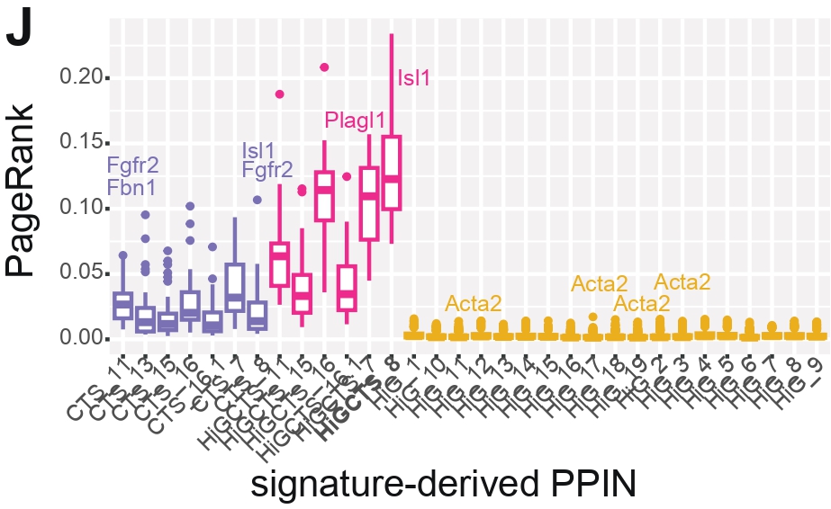
Panel J — Boxplot of PageRank per PPIN
Purpose
To show the full distribution of PageRank values across all genes in each PPIN, complementing the median-based view from Panel C.
What this Panel Shows
Boxplot of PageRank for each PPIN.
CHD-risk genes labeled when ranked in the top 5 by PageRank.
Interpretation
PageRank analysis shows that, in CTS and CTS&HiG PPINs, only a small number of genes stand out as especially
influential within the network, even though these networks do not rely on a single dominant hub overall.
These influential genes sit at key positions in transition networks, where changes to them could have broad
effects on how signals propagate across the system. By contrast, HiG PPINs display consistently low PageRank
values across genes, suggesting a network structure driven more by tightly connected local groups than by a
few genes with system-wide influence.
Inputs
df_PAGERANK_strength_ANND.rewring.P.rds
CHD_Cilia_Genelist.rds
Outputs
Note: figures shown are polished versions of the raw outputs
###################################################
# Fig J) boxplot of PageRank per PPIN
# original code: Code: 11.3_CTS_cardiac_network_ANND_pagerank.R
# original pdf: PageRank_GSE870383_v2.pdf
################################################################
{
CHD = readRDS( file=paste0(inputdir, 'CHD_Cilia_Genelist.rds'))

df = readRDS(file='df_PAGERANK_strength_ANND.rewring.P.rds')  #!!!!!!!!!!!!!!!!!!!!!!!

df = rbind(subset(df, PPI_cat=='CTS'),
                    subset(df, PPI_cat=='HiGCTS'),
                    subset(df, PPI_cat=='HiG')
                    )
## ensure the same order along x-axis
# df$signature <- factor(df$signature, levels = signature_levels)
df$label=df$gene
df$PCGC_AllCurated = toupper(df$gene) %in% toupper(unlist(CHD['Griffin2023_PCGC_AllCurated']))
# Calculate top 5 significant genes within each box
df5 <- df %>%
        filter(rank_by_PR <= 5) %>%
        ungroup()
tb = df5[, c('signature','gene','PPI_cat','rank_by_PR','PCGC_AllCurated')]
write.table(tb, file= 'table_top5_pagerank_perPPI.tsv', sep='\t', row.names=F)

df5_CHD = subset(df5, PCGC_AllCurated==TRUE)
(dim(df5_CHD))  # [1] 15 18

boxplot_pagerank <- ggplot(df, aes(x = signature, y = PageRank, colour = PPI_cat)) +
    geom_boxplot(show.legend = TRUE) + # Enable legend for the boxplot
    scale_color_manual(values = PPI_color_palette) +
    geom_text(
        data = df5_CHD, aes(label = gene), # data=df5
        size = 2, # Adjust the size of the text labels
        hjust = -0.1, vjust = 0,
        check_overlap = TRUE
    ) + # Avoid text overlap
    theme(
        legend.position = "none", # c(1, 1),
        legend.justification = c(1, 1), # Place legend at top-right corner
        axis.text.x = element_text(angle = 45, vjust = 1, hjust = 1)
    ) +
    scale_x_discrete(limits = unique(df$signature)) +
    labs(color = "PPI cat") # Optional: label for the color legend

vertex(boxplot_pagerank)
}
Appendix — Derived Data Used in Panels
Panel A & B & C(left) — Strength Architecture and Distribution
Weighted graphs (GSE87038_STRING_graph_perState_simplified_combinedweighted.rds)
created by code/11.2.0_update_network_weights_clean_max.R. Refer to Appendix — Key File Lineage Prior to 11.2.0 for more information
Node strength was computed, normalized, and consolidated with PageRank and ANND results by rewiring test in
code/11.3_CTS_cardiac_network_ANND_pagerank.R, producing
df_PAGERANK_strength_ANND.rewring.P.rds.
Weighted graphs (GSE87038_STRING_graph_perState_simplified_combinedweighted.rds)
created by code/11.2.0_update_network_weights_clean_max.R. Refer to Appendix — Key File Lineage Prior to 11.2.0 for more information